Edge Coupled Stripline Impedance
PCB Differential Stripline Impedance Calculator
Differential Stripline Impedance Calculator
Choose Type
Edge Coupled Stripline Impedance Calculator
Inputs
Outputs
Introduction
The edge couple differential symmetric stripline transmission line is a common technique for routing differential traces. There are four different types of impedance used in characterizing differential trace impedances. This calculator finds both odd and even transmission line impedance. Modeling approximation can be used to understand the impedance of the edge couple differential stripline transmission line.
Description
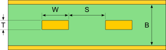
An edge couple differential symmetric stripline transmission line is constructed with two traces referenced to the same reference planes above and below the traces. There is a dielectric material between them. There is also some coupling between the lines. This coupling is one of the features of differential traces. Usually it is good practice to match differential trace length and to keep the distances between the traces consistent. Also avoid placing vias and other structures between these traces.
Differential Impedance Definitions
Differential Impedance The impedance measured between the two lines when they are driven with opposite polarity signals. Zdiff is equal to twice the value of Zodd
Odd Impedance The impedance measured when testing only one of the differential traces referenced to the ground plane. The differential signals need to be driven with opposite polarity signals. Zodd is equal to half of the value of Zdiff
Common Impedance The impedance measured between the two lines when they are driven with the same signal. Zcommon is half the value of Zeven
Even Impedance The impedance measured when testing only one of the differential traces referenced to the ground plane. The differential signals need to be driven with the same identical signal. Zeven is twice the value of Zcommon
Microstrip Transmission Line Models
Models have been created to approximate the characteristics of the microstrip transmission line.
h=\frac{b-t}{2}
ke=\tanh \left ( \frac{\pi w}{2b} \right )\cdot \tanh \left ( \frac{\pi }{2}\cdot\frac{w+s}{b} \right )
ko=\tanh \left ( \frac{\pi w}{2b} \right )\cdot \coth \left ( \frac{\pi }{2}\cdot\frac{w+s}{b} \right )
k_{e}^{`}=\sqrt{1-ke^{2}}
k_{o}^{`}=\sqrt{1-ko^{2}
z_{o,e}=\frac{30\pi }{\sqrt{er}}\cdot \frac{K(k_{e}^{`})}{K(k_{e})}
z_{o,o}=\frac{30\pi }{\sqrt{er}}\cdot \frac{K(k_{o}^{`})}{K(k_{o})}
Z_{o,ss}=symmetric\:stripline(w,t,h,er)
C_{f}^{`}\left ( \frac{t}{b} \right )=\frac{.0885\eta_{r}}{\pi }\left \{ \frac{2b}{b-t}\ln \left ( \frac{2b-t}{b-t} \right )-\left ( \frac{t}{b-t} \right )\ln \left ( \frac{b^{2}}{\left ( b-t \right )^{2}}-1 \right ) \right \}
C_{f}^{`}\left ( 0 \right )=\frac{.0885e_{r}}{\pi }\cdot 2\ln \left ( 2 \right )
k_{ideal}=\text sech\left ( \frac{\pi w}{2b} \right )
k_{ideal}^{`}=\text tanh\left ( \frac{\pi w}{2b} \right )